
Note
Click here to download the full example code
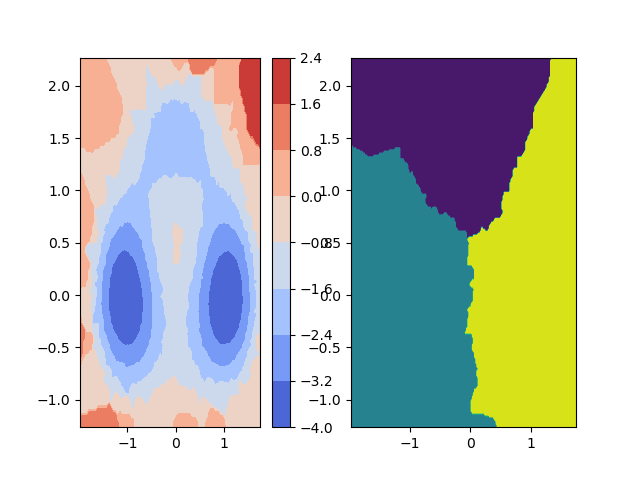
2D contours from xyz
This example demonstrates how to plot unordered xyz data - in this case, particle positions (xy) and their energy (z) -
as contour as well as a state map on the right-hand side depicting a decomposition into three coarse metastable states.
See deeptime.plots.plot_contour2d_from_xyz().
10 import numpy as np
11
12 import matplotlib.pyplot as plt
13
14 from deeptime.clustering import KMeans
15 from deeptime.markov.msm import MaximumLikelihoodMSM
16
17 from deeptime.data import triple_well_2d
18 from deeptime.plots import plot_contour2d_from_xyz
19
20 system = triple_well_2d(h=1e-3, n_steps=100)
21 trajs = system.trajectory(x0=[[-1, 0], [1, 0], [0, 0]], length=5000)
22 traj_concat = np.concatenate(trajs, axis=0)
23
24 energies = system.potential(traj_concat)
25
26 clustering = KMeans(n_clusters=20).fit_fetch(traj_concat)
27 dtrajs = [clustering.transform(traj) for traj in trajs]
28
29 msm = MaximumLikelihoodMSM(lagtime=1).fit(dtrajs).fetch_model()
30 pcca = msm.pcca(n_metastable_sets=3)
31 coarse_states = pcca.assignments[np.concatenate(dtrajs)]
32
33 f, (ax1, ax2) = plt.subplots(1, 2)
34 ax1, mappable = plot_contour2d_from_xyz(*traj_concat.T, energies, contourf_kws=dict(cmap='coolwarm'), ax=ax1)
35 ax2, _ = plot_contour2d_from_xyz(*traj_concat.T, coarse_states, n_bins=200, ax=ax2)
36 f.colorbar(mappable, ax=ax1)
Total running time of the script: ( 0 minutes 0.860 seconds)
Estimated memory usage: 22 MB