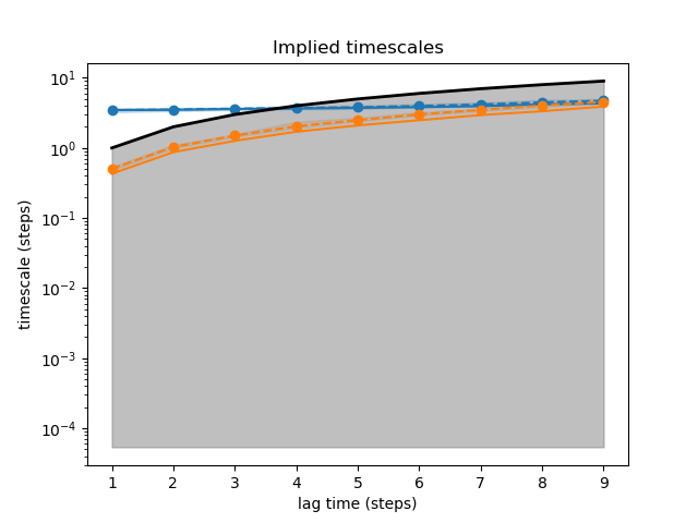
Implied timescales

This example demonstrates how to obtain an implied timescales (ITS) plot for a Bayesian Markov state model.

import matplotlib.pyplot as plt
import numpy as np

from deeptime.clustering import KMeans
from deeptime.data import double_well_2d
from deeptime.markov import TransitionCountEstimator
from deeptime.markov.msm import BayesianMSM
from deeptime.plots import plot_implied_timescales
from deeptime.util.validation import implied_timescales

system = double_well_2d()
data = system.trajectory(x0=np.random.normal(scale=.2, size=(10, 2)), length=1000)
clustering = KMeans(n_clusters=50).fit_fetch(np.concatenate(data))
dtrajs = [clustering.transform(traj) for traj in data]

models = []
lagtimes = np.arange(1, 10)
for lagtime in lagtimes:
    counts = TransitionCountEstimator(lagtime=lagtime, count_mode='effective').fit_fetch(dtrajs)
    models.append(BayesianMSM(n_samples=50).fit_fetch(counts))

its_data = implied_timescales(models)

fig, ax = plt.subplots(1, 1)
plot_implied_timescales(its_data, n_its=2, ax=ax)
ax.set_yscale('log')
ax.set_title('Implied timescales')
ax.set_xlabel('lag time (steps)')
ax.set_ylabel('timescale (steps)')

Estimated memory usage: 9 MB