function quadruple_well_asymmetric

deeptime.data.quadruple_well_asymmetric(h=0.001, n_steps=10000)

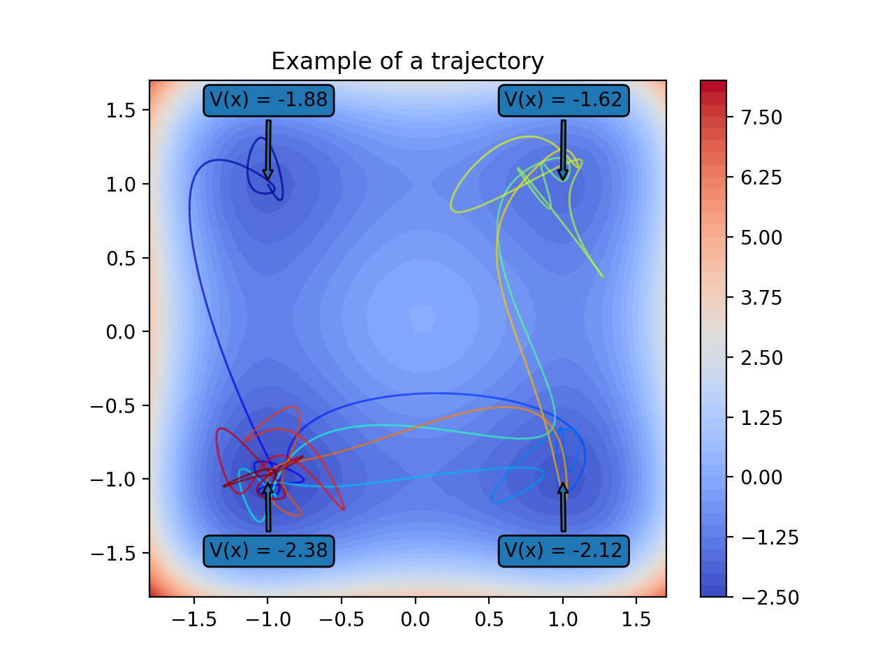
This dataset generates trajectories of a two-dimensional particle living in an asymmetric quadruple-well potential landscape. It is subject to the stochastic differential equation

\[\mathrm{d}X_t = \nabla V(X_t) \mathrm{d}t + \sigma\mathrm{d}W_t\]

with \(W_t\) being a Wiener process and the potential \(V\) being given by

\[V(x) = (x_1^4-\frac{x_1^3}{16}-2x_1^2+\frac{3x_1}{16}) + (x_2^4-\frac{x_1^3}{8}-2x_1^2+\frac{3x_1}{8}).\]

The stochastic force parameter is set to \(\sigma = 0.6\).

(Source code, png, hires.png, pdf)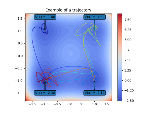

Parameters:

• h (float, default = 1e-3) – Integration step size. The implementation uses an Euler-Maruyama integrator.

• n_steps (int, default = 10000) – Number of integration steps between each evaluation. That means the default lag time is h*n_steps=10.

Returns:

model – The model.

Return type:

TimeIndependentSystem

Examples

The model possesses the capability to simulate trajectories as well as be evaluated at test points:

>>> import numpy as np
>>> import deeptime as dt

First, set up the model (which internally already creates the integrator).

>>> model = dt.data.quadruple_well_asymmetric(h=1e-3, n_steps=100)  # create model instance

Now, a trajectory can be generated:

>>> traj = model.trajectory(np.array([[0., 0.]]), 1000, seed=42, n_jobs=1)  # simulate trajectory
>>> assert traj.shape == (1000, 2)  # 1000 evaluations from initial condition [0, 0]

Or, alternatively the model can be evaluated at test points (mapping forward using the dynamical system):

>>> test_points = np.random.uniform(-2, 2, (100, 2))  # 100 test point in [-2, 2] x [-2, 2]
>>> evaluations = model(test_points, seed=53, n_jobs=1)
>>> assert evaluations.shape == (100, 2)