
function prinz_potential
- deeptime.data.prinz_potential(h=1e-05, n_steps=500, temperature_factor=1.0, mass=1.0, damping=1.0)
Particle diffusing in a one-dimensional quadruple well potential landscape. [1]
The potential is defined as
\[V(x) = 4 \left( x^8 + 0.8 e^{-80 x^2} + 0.2 e^{-80 (x-0.5)^2} + 0.5 e^{-40 (x+0.5)^2}\right). \]The integrator is an Euler-Maruyama type integrator, updating the current state \(x_t\) via
\[x_{t+1} = x_t - \frac{h\nabla V(x_t)}{m\cdot d} + \sqrt{2\frac{h\cdot\mathrm{kT}}{m\cdot d}}\eta_t, \]where \(m\) is the mass, \(d\) the damping factor, and \(\eta_t \sim \mathcal{N}(0, 1)\).
The locations of the minima can be accessed via the minima attribute.
(
Source code,png,hires.png,pdf)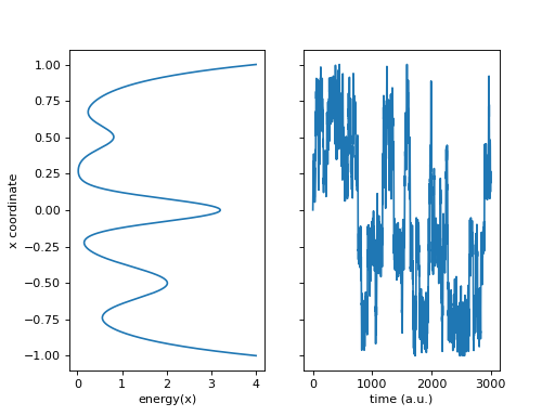
- Parameters:
h (float, default=1e-5) – The integrator step size. If the temperature is too high and the step size too large, the integrator may produce NaNs.
n_steps (int, default=500) – Number of integration steps between each evaluation of the system’s state.
temperature_factor (float, default=1) – The temperature kT.
mass (float, default=1) – The particle’s mass.
damping (float, default=1) – Damping factor.
- Returns:
system – The system.
- Return type:
Examples
The model possesses the capability to simulate trajectories as well as be evaluated at test points:
>>> import numpy as np
>>> from deeptime.data import prinz_potential
First, set up the model (which internally already creates the integrator).
>>> model = prinz_potential(h=1e-3, n_steps=100) # create model instance
Now, a trajectory can be generated:
>>> traj = model.trajectory(np.array([[-0.]]), 1000, seed=42, n_jobs=1)  # simulate trajectory
>>> assert traj.shape == (1000, 1)  # 1000 evaluations from initial condition [0]
Or, alternatively the model can be evaluated at test points (mapping forward using the dynamical system):
>>> test_points = np.random.uniform(.5, 1.5, (100, 1))  # 100 test points
>>> evaluations = model(test_points, seed=53, n_jobs=1)
>>> assert evaluations.shape == (100, 1)
We can obtain the x-coordinates of the energy minima via the minima attribute:
>>> model.minima
array([-0.73943019, -0.22373758,  0.26914935,  0.67329635])
References