Transition counting

To begin estimating markov state models one needs to collect statistics over available data, in particular transitions between states at a given lag time \(\tau\).

These statistics can be collected using deeptime’s transition count estimator (apidocs).

When creating an instance of said estimator, one has to make two choices: The lagtime \(\tau > 0\) and the count mode. The lag time is the step size of the markov chain, i.e, an underlying transition matrix of the process with

\[P_{ij} = \mathbb{P}(X_{t+\tau}=j \mid X_t = i). \]

The count mode can be one of:

• "sample": Strides the trajectory with lagtime \(\tau\) and uses the strided counts as transitions, i.e., a trajectory of length \(T\) has \(\lfloor T/\tau \rfloor\) counts at time indices

  \[(0 \rightarrow \tau), (\tau \rightarrow 2 \tau), ..., (((T/ \tau )-1) \tau \rightarrow T). \]

  This means that potentially transitions can be missed.

• "sliding": Uses a sliding window approach for counting. A trajectory of length \(T\) has \(T-\tau\) transition counts at

  \[(0 \rightarrow \tau), (1 \rightarrow \tau+1), ..., (T-\tau-1 \rightarrow T-1). \]

  This introduces an overestimation of the actual count values by a factor of “lagtime”. For maximum-likelihood MSMs this plays no role but it leads to wrong error bars in uncertainty estimation.

• "sliding-effective": Same as sliding mode, just that the resulting count matrix is divided by the lagtime after counting. This which can be shown to provide a likelihood that is the geometrical average over shifted subsamples of the trajectory, \((s_1,\:s_{tau+1},\:...),\:(s_2,\:t_{tau+2},\:...)\), etc. This geometrical average converges to the correct likelihood in the statistical limit [1].

• "effective": Uses an estimate of the transition counts that are statistically uncorrelated. Recommended when used with a Bayesian MSM (or the respective API docs). A description of the estimation procedure can be found in [2].

import numpy as np
from deeptime.markov import TransitionCountEstimator

estimator = TransitionCountEstimator(
    lagtime=1,
    count_mode="sliding"
)

The estimator can be used to fit a count model:

trajectory = np.array([0, 1, 2, 3, 4, 5, 4, 3, 2, 1, 0, 1, 2, 3, 4, 5, 6, 5, 4, 3, 2, 1, 7])
counts = estimator.fit(trajectory).fetch_model()  # fit and fetch the model

The count model has several properties, which can be used to later on estimate markov state models. One of them is the count matrix \(C\), which countains transition counts from one state to the other as encountered in the trajectory:

counts.count_matrix

array([[0., 2., 0., 0., 0., 0., 0., 0.],
       [1., 0., 2., 0., 0., 0., 0., 1.],
       [0., 2., 0., 2., 0., 0., 0., 0.],
       [0., 0., 2., 0., 2., 0., 0., 0.],
       [0., 0., 0., 2., 0., 2., 0., 0.],
       [0., 0., 0., 0., 2., 0., 1., 0.],
       [0., 0., 0., 0., 0., 1., 0., 0.],
       [0., 0., 0., 0., 0., 0., 0., 0.]])

In this example, the \((1,2)\)-th element is \(C_{12} = 2\), meaning there are two counted transitions from state \(1\) to state \(2\). Furthermore, one has access to a state histogram, which contains the information how often each state was visited within the presented data.

for state, histogram_value in enumerate(counts.state_histogram):
    print(f"State {state}: {histogram_value} occurances.")

State 0: 2 occurances.
State 1: 4 occurances.
State 2: 4 occurances.
State 3: 4 occurances.
State 4: 4 occurances.
State 5: 3 occurances.
State 6: 1 occurances.
State 7: 1 occurances.

Selecting a submodel

Depending on what kind of markov model is estimated, it is required to have either a strongly or weakly connected set of states. This means that the count matrix is interpreted as an adjacency matrix

\[A_{ij} = \begin{cases}1 &\text{, if } C_{ij} > 0 \\ 0 &\text{, otherwise.}\end{cases} \]

A graph induced by the adjacency matrix is called strongly connected if the edges are directed and there is a path from each state \(i\) to each state \(j\). It is called weakly connected if the edges are undirected and there is a path from each state \(i\) to each state \(j\).

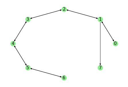
Plotting the graph (using networkx), one can see that our example data consists of \(8\) states in total where all except state \(7\) are strongly connected.

import matplotlib.pyplot as plt
import networkx as nx

G = nx.from_numpy_matrix(counts.count_matrix, create_using=nx.DiGraph())
pos = nx.circular_layout(G)
nx.draw_circular(G, node_color='#90EE90')
nx.draw_networkx_labels(G, pos, labels={i: i for i in G.nodes()}, font_size=15)
plt.show()

The connected sets (weak and strong) can be obtained from the model directly:

print("Weakly connected sets:", counts.connected_sets(directed=False))
print("Strongly connected sets:", counts.connected_sets(directed=True))

Weakly connected sets: [array([0, 1, 2, 3, 4, 5, 6, 7])]
Strongly connected sets: [array([0, 1, 2, 3, 4, 5, 6]), array([7])]

And a submodel can be selected based on either an explicitly selected subset of states:

submodel_explicit = counts.submodel(states=[0, 1, 7])

Which then contains a subselected count matrix. The “states” of a count model always refer to the dimensions of the count matrix, i.e., if \(C\in\mathbb{R}^{n\times n}\), then there are \(n\) states. To be able to trace back, which state in a submodel belongs to which state in the data, there are also “symbols”, which are the states of the root model:

print("# states:", submodel_explicit.n_states)
print("symbols:", submodel_explicit.state_symbols)

# states: 3
symbols: [0 1 7]

If presented with a set of symbols which should be mapped to states, there is a convenience function (no longer present symbols are discarded):

submodel_explicit.symbols_to_states([0, 1, 7, 8])

array([0, 1, 2])

Furthermore one can restrict data to the state selection of the model. No longer present symbols are set to -1:

submodel_explicit.transform_discrete_trajectories_to_submodel(trajectory)

[array([ 0,  1, -1, -1, -1, -1, -1, -1, -1,  1,  0,  1, -1, -1, -1, -1, -1,
        -1, -1, -1, -1,  1,  2], dtype=int32)]

Most of the time the state selection should be based on the connected sets. For this, one can call

submodel = counts.submodel_largest(connectivity_threshold=1., directed=True)

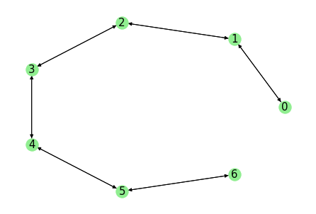
This selects the largest (strongly) connected set where only states with at least 1 transition count are considered connected.

G = nx.from_numpy_matrix(submodel.count_matrix, create_using=nx.DiGraph())
pos = nx.circular_layout(G)
nx.draw_circular(G, node_color='#90EE90')
nx.draw_networkx_labels(G, pos, labels={i: i for i in G.nodes()}, font_size=15)
plt.show()

As one can see, the weakly connected state 7 is removed.

Optionally, one can give probability constraints of states as well as selected the connected set by population and not by size. A description of this can be found here.

References

[1]

Benjamin Trendelkamp-Schroer, Hao Wu, Fabian Paul, and Frank Noé. Estimation and uncertainty of reversible markov models. The Journal of chemical physics, 143(17):11B601_1, 2015.

[2]

Frank Noé. Statistical inefficiency of markov model count matrices. Preprint, http://publications. mi. fu-berlin. de/1699, 2015.