Maximum-likelihood MSMs

For those already familiar with the interface: The corresponding API docs.

This kind of estimator tries to determine the most likely transition matrix \(P\in\mathbb{R}^{n\times n}\) given the transition counts \(C\in\mathbb{R}^{n\times n}\) [1][2].

The likelihood that a transition matrix \(P\) belongs to a trajectory \(S = (s_0,\ldots,s_T)\) is given by

\[\mathcal{L}(P) = \mathbb{P}(P\mid S) = \prod_{i,j=1}^n P_{ij}^{C_{ij}}. \]

After importing the package, the estimator can be instantiated:

import deeptime.markov as markov

estimator = markov.msm.MaximumLikelihoodMSM(
    reversible=True,
    stationary_distribution_constraint=None
)

It has two main parameters:

• reversible determines whether the estimated MSM should have a detailed balance symmetry, i.e.,

  \[\pi_i P_{ij} = \pi_j P_{ji}\quad\forall i,j=1,\ldots,n, \]

  where \(\pi\) is the stationary probability distribution vector. It is the probability vector which does not change under \(P\), i.e., \(P\pi = \pi\) and therefore is eigenvector for eigenvalue \(\lambda_0\) = 1. A sufficient condition for existence and uniqueness of \(\pi\) is the irreducibility of the markov chain, i.e., the count matrix must be connected.

• stationary_distribution_constraint: In case the stationary distribution \(\pi\) is known a priori, the search space can be restricted to stochastic matrices which have \(\pi\) as stationary distribution.

To demonstrate the estimator, we can generate a sequence of observations from a markov state model. It has three states and a probability of \(97\%\) to stay in its current state. The remaining \(3\%\) are used as jump probabilities.

import numpy as np

p11 = 0.97
p22 = 0.97
p33 = 0.97
P = np.array([[p11, 1 - p11, 0], [.5*(1 - p22), p22, 0.5*(1-p22)], [0, 1-p33, p33]])
true_msm = markov.msm.MarkovStateModel(P)

A realization of this markov state model can be generated:

trajectory = true_msm.simulate(50000)

And we can gather statistics about it

counts_estimator = markov.TransitionCountEstimator(
    lagtime=1, count_mode="sliding"
)
counts = counts_estimator.fit(trajectory).fetch_model()

as well as re-estimate an MSM.

msm = estimator.fit(counts).fetch_model()

The estimated transition matrix is reasonably close to the ground truth:

print("Estimated transition matrix:", msm.transition_matrix)
print("Estimated stationary distribution:", msm.stationary_distribution)

Estimated transition matrix: [[0.97174192 0.02825808 0.        ]
 [0.01436794 0.97057023 0.01506183]
 [0.         0.02829029 0.97170971]]
Estimated stationary distribution: [0.24913759 0.48999019 0.26087221]

Now since we know the stationary distribution of the ground truth, we can restrict the estimator’s optimization space to it:

print("True stationary vector:", true_msm.stationary_distribution)

True stationary vector: [0.25 0.5  0.25]

estimator.stationary_distribution_constraint = true_msm.stationary_distribution

msm_statdist = estimator.fit(counts).fetch_model()

print("Estimated transition matrix:", msm_statdist.transition_matrix)
print("Estimated stationary distribution:", msm_statdist.stationary_distribution)

Estimated transition matrix: [[0.97150033 0.02849967 0.        ]
 [0.01424983 0.97116296 0.0145872 ]
 [0.         0.0291744  0.9708256 ]]
Estimated stationary distribution: [0.25 0.5  0.25]

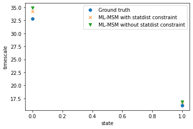
With the markov state model object one also has access to relaxation timescales \(t_s = -\tau / \mathrm{ln} | \lambda_i |, i = 2,...,k+1\):

import matplotlib.pyplot as plt

plt.plot(true_msm.timescales(), 'o', label="Ground truth")
plt.plot(msm_statdist.timescales(), 'x', label="ML-MSM with statdist constraint")
plt.plot(msm.timescales(), 'v', label="ML-MSM without statdist constraint")
plt.xlabel("state")
plt.ylabel("timescale")
plt.legend();

Bayesian sampling

While the maximum likelihood estimation is useful, it does not say anything about uncertainties. These can be obtained by estimating a Bayesian posterior with the Bayesian MSM [3]. The posterior contains the prior around which sampling was performed as well as samples over which statistics can be collected.

Similarly to the maximum-likelihood estimator it has the option to make estimation reversible as well as to introduce a stationary_distribution_constraint. Furthermore, it can be specified how many samples should be drawn as well as how many Gibbs sampling should be performed for each output sample.

estimator = markov.msm.BayesianMSM(
    n_samples=100,
    n_steps=10,
    reversible=True,
    stationary_distribution_constraint=None
)

To fit the model, an effective counting should be used as sliding window counting leads to wrong uncertainties.

counts_estimator = markov.TransitionCountEstimator(
    lagtime=1, count_mode="effective"
)
counts_effective = counts_estimator.fit(trajectory).fetch_model()

With the estimated effective counts, we are ready to estimate the posterior.

bmsm_posterior = estimator.fit(counts_effective).fetch_model()

The prior can be accessed via the prior property, the samples can be accessed via the samples property. Both are just instances of MarkovStateModel and a list thereof, respectively.

print("# samples:", len(bmsm_posterior.samples))

# samples: 100

The posterior instance also offers a method to gather statistics over all evaluatable methods of the markov state model. Just put the name of method or property as a string, if it is a method of something that is returned by another method, just separate with a /. Below a few examples:

stats_P = bmsm_posterior.gather_stats("transition_matrix")
stats_timescales = bmsm_posterior.gather_stats("timescales")
stats_C = bmsm_posterior.gather_stats("count_model/count_matrix")

If a quantity evaluation requires arguments, they can be attached to the gather_stats method:

stats_mfpt = bmsm_posterior.gather_stats("mfpt", A=0, B=1)

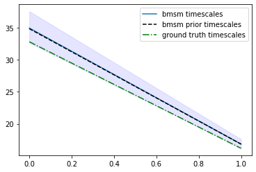
These statistics contain mean, standard deviation, as well as confidence intervals.

plt.plot([0, 1], stats_timescales.mean, label="bmsm timescales")
plt.fill_between([0, 1], stats_timescales.L, stats_timescales.R, color='b', alpha=.1)
plt.plot([0, 1], bmsm_posterior.prior.timescales(), "k--", label="bmsm prior timescales")
plt.plot([0, 1], true_msm.timescales(), "g-.", label="ground truth timescales")
plt.legend();

To, e.g., visualize samples differently or evaluate other kinds of moments, one can get access to the evaluated quantities directly by setting store_samples to True:

stats_mfpt = bmsm_posterior.gather_stats("mfpt", store_samples=True, A=0, B=1)
print("# samples:", len(stats_mfpt.samples))

# samples: 100

References

[1]

Ch Schütte, Alexander Fischer, Wilhelm Huisinga, and Peter Deuflhard. A direct approach to conformational dynamics based on hybrid monte carlo. Journal of Computational Physics, 151(1):146–168, 1999.

[2]

Hao Wu and Frank Noé. Variational approach for learning markov processes from time series data. Journal of Nonlinear Science, 30(1):23–66, 2020.

[3]

Benjamin Trendelkamp-Schroer, Hao Wu, Fabian Paul, and Frank Noé. Estimation and uncertainty of reversible markov models. The Journal of chemical physics, 143(17):11B601_1, 2015.