
Note
Go to the end to download the full example code.
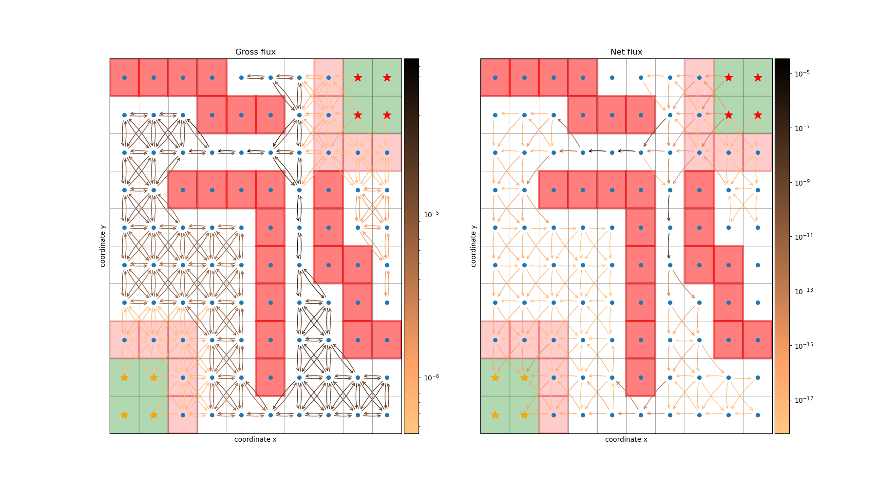
Gross and net flux on the Drunkard’s walk
This example shows how to compute and visualize gross and net reactive flux (see deeptime.markov.ReactiveFlux)
using the deeptime.data.drunkards_walk().
 9 import matplotlib as mpl
10 import matplotlib.pyplot as plt
11 from mpl_toolkits.axes_grid1 import make_axes_locatable
12
13 import numpy as np
14
15 from deeptime.data import drunkards_walk
16
17 sim = drunkards_walk(grid_size=(10, 10),
18                      bar_location=[(0, 0), (0, 1), (1, 0), (1, 1)],
19                      home_location=[(8, 8), (8, 9), (9, 8), (9, 9)])
20 sim.add_barrier((5, 1), (5, 5))
21 sim.add_barrier((0, 9), (5, 8))
22 sim.add_barrier((9, 2), (7, 6))
23 sim.add_barrier((2, 6), (5, 6))
24
25 sim.add_barrier((7, 9), (7, 7), weight=5.)
26 sim.add_barrier((8, 7), (9, 7), weight=5.)
27
28 sim.add_barrier((0, 2), (2, 2), weight=5.)
29 sim.add_barrier((2, 0), (2, 1), weight=5.)
30
31 flux = sim.msm.reactive_flux(sim.home_state, sim.bar_state)
32
33 fig, axes = plt.subplots(1, 2, figsize=(18, 10))
34 dividers = [make_axes_locatable(axes[i]) for i in range(len(axes))]
35 caxes = [divider.append_axes("right", size="5%", pad=0.05) for divider in dividers]
36
37 titles = ["Gross flux", "Net flux"]
38 fluxes = [flux.gross_flux, flux.net_flux]
39
40 cmap = plt.cm.copper_r
41 thresh = [0, 1e-12]
42
43 for i in range(len(axes)):
44     ax = axes[i]
45     F = fluxes[i]
46     ax.set_title(titles[i])
47
48     vmin = np.min(F[np.nonzero(F)])
49     vmax = np.max(F)
50
51     sim.plot_2d_map(ax)
52     sim.plot_network(ax, F, cmap=cmap, connection_threshold=thresh[i])
53     norm = mpl.colors.LogNorm(vmin=vmin, vmax=vmax)
54     fig.colorbar(plt.cm.ScalarMappable(norm=norm, cmap=cmap), cax=caxes[i])
Total running time of the script: (0 minutes 0.753 seconds)
Estimated memory usage: 590 MB