DMD¶

For people already familiar with the method and interface, the API docs.

Here we present the basic ideas behind a family of dynamic mode decomposition (DMD) methods. In particular the original “standard DMD” [1], its variant “exact DMD” [2]. The principle idea is that DMD should be able to characterize / decompose potentially highly nonlinear dynamics by solving linear systems of equations and studying their spectral properties.

Considering a sequential set of data vectors \(\{z_1,\ldots,z_m\}\) with \(z_i\in\mathbb{R}^n\) and assuming that

\[z_{k+1} = Az_k \]

for some usually unknown matrix \(A\), one can define standard DMD as follows (following the presentation of [2], originally introduced as DMD in [1] ).

The data is arranged into matrices \(X, Y\) of matching pairs of time-shifted datapoints, i.e., \(Y_{i+1} = X_{i}\) for \(i \geq 1\).
Compute the (optionally truncated) SVD of \(X\) to obtain \(X = U\Sigma V^*\).
Define \(\tilde{A} = U^*YV\Sigma^{-1}\).
Compute eigenvalues and eigenvectors \(\tilde A w = \lambda w\).
The DMD mode corresponding to the DMD eigenvalue \(\lambda\) is given by \(\hat\varphi = Uw\).

It should be remarked that even if the data-generating dynamics are nonlinear, it is assumed that there exists some linear operator \(A\) which approximates these.

The notion of “exact” DMD [2] weakens the assumptions and only requires that the data vectors are corresponding pairs of data. The operator \(A\) is defined as the solution to the best-approximation of \(\| AX - Y\|_F\). This leads to exact DMD modes corresponding to eigenvalue \(\lambda\) of the form

\[\varphi = \frac{1}{\lambda}YV\Sigma^{-1}w. \]

Both estimation modes are united within the same estimator in Deeptime:

[1]:

from deeptime.decomposition import DMD

standard_dmd = DMD(mode='standard')
exact_dmd = DMD(mode='exact')

The standard DMD is sometimes also referred to as projected DMD [2] since the modes \(\hat\varphi\) are eigenvectors of \(\mathbb{P}_XA\), where \(\mathbb{P}_X = UU^*\) is the orthogonal projection onto the image of \(X\). If data vectors \(y_i\) are in the \(\mathrm{span}\{x_i\}\), then \(\mathbb{P}_X = \mathrm{Id}\); projected/standard and exact DMD modes coincide.

This can be especially relevant if there are more dimensions than datapoints.

We demonstrate the methods using a random orthogonal matrix \(A\) which serves as out propagator plus some normal distributed noise, i.e.,

\[x_{t+1} = Ax_t + \mathcal{N}(0, 10^{-4}). \]

[2]:

import numpy as np

state = np.random.RandomState(45)

A = np.linalg.qr(state.normal(size=(2, 2)))[0]
x0 = state.uniform(-1, 1, size=(A.shape[0],))

data = np.empty((500, A.shape[0]))
data[0] = x0
for t in range(1, len(data)):
    data[t] = A @ data[t - 1] + state.normal(scale=1e-4, size=(2,))

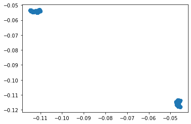
Visualizing the generated data we can see that it is a jumping process between two wells.

[3]:

import matplotlib.pyplot as plt
plt.scatter(*data.T);

Fitting the models to this dataset reveals that the eigenvalues are identical:

[4]:

standard_model = standard_dmd.fit((data[:-1], data[1:])).fetch_model()
exact_model = exact_dmd.fit((data[:-1], data[1:])).fetch_model()

[5]:

print(f"Eigenvalues standard {standard_model.eigenvalues}, exact {exact_model.eigenvalues}")

Eigenvalues standard [ 1.00003048+0.j -1.00015445+0.j], exact [ 1.00003048+0.j -1.00015445+0.j]

We propagate the first ten datapoints using our estimated models:

[6]:

traj_standard = standard_model.transform(data)
traj_exact = exact_model.transform(data)

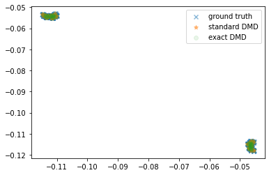
A scatter plot reveals that all data points get mapped to the same two wells and the propagator was approximated almost perfectly.

[7]:

plt.scatter(*data.T, alpha=.5, marker='x', label='ground truth')
plt.scatter(*np.real(traj_standard)[::5].T, marker='*',alpha=.5, label='standard DMD')
plt.scatter(*np.real(traj_exact)[::5].T, alpha=.1, label='exact DMD')
plt.legend();

References