Kernel EDMD

This notebook illustrates how to use kernel extended dynamic mode decomposition (kernel EDMD) [1] to compute eigenfunctions of the Koopman operator and Perron-Frobenius operator.

An alternative derivation of kernel EDMD using covariance and cross-covariance operators defined on reproducing kernel Hilbert spaces, highlighting also relationships with conditional mean embeddings of distributions and the Perron-Frobenius operator, is presented in [2]. High-dimensional molecular dynamics problems can be found in [3].

Given training data $\{x_i\}_{i=1}^m$ and $\{y_i\}_{i=1}^m$, where $y_i$ is a time-lagged version of $x_i$, let $\varphi$ denote an eigenfunction and $\lambda$ the corresponding eigenvalue. For the Perron-Frobenius operator, we obtain kernel-based approximations of eigenvalues and eigenfunctions by

$$(G_{XX}+m\varepsilon I)^{-1}G_{XY} \mathbf{v} = \lambda \mathbf{v}, \quad \varphi = \Phi G_{XX}^{-1} \mathbf{v}$$

and for the Koopman operator by

$$(G_{XX} + m \varepsilon I)^{-1} G_{YX} \mathbf{v} = \lambda \mathbf{v}, \quad \varphi = \Phi \mathbf{v},$$

where $\Phi=[\phi(x_1), \dots, \phi(x_m)]$ is the so-called feature matrix and $\varepsilon$ a regularization parameter. The matrices $G_{XX}$ and $G_{XY}$ are the standard Gram matrix and the time-lagged Gram matrix, respectively, with entries $[G_{XX}]_{ij} = k(x_i, x_j)$ and $[G_{XY}]_{ij} = k(x_i, y_j)$. Moreover, $G_{YX}=G_{XY}^\top$.

import numpy as np
import matplotlib.pyplot as plt

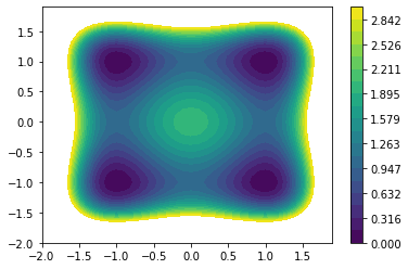
First we define a dynamical system. We will use a quadruple-well problem as our guiding example, which is given by a stochastic differential equation of the form

$$\mathrm{d}X_t = -\nabla V(X_t) \mathrm{d}t + \sqrt{2 \beta^{-1}} \mathrm{d}W_t.$$

The potential $V$ is defined by

$$V(x) = (x_1^2 - 1)^2 + (x_2^2 - 1)^2 .$$

We define the inverse temperature to be $\beta = 4$. Let us visualize the potential.

xy = np.arange(-2, 2, 0.1)
XX, YY = np.meshgrid(xy, xy)
V = (XX**2 - 1)**2 + (YY**2 - 1)**2
plt.contourf(xy, xy, V, levels=np.linspace(0.0, 3.0, 20))

plt.colorbar();

The dynamical system itself is implented in C++ for the sake of efficiency. The SDE is solved with the Euler-Maruyama method.

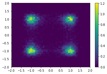
To visualize the system’s dynamics we generate one long trajectory and plot a histogram. The density is high where the potential is low and vice versa. A particle will typically stay in one well for a long time before it transitions to other wells. There are thus four metastable states corresponding to the four wells.

We can load the model as follows.

from deeptime.data import quadruple_well

h = 1e-3 # step size of the Euler-Maruyama integrator
n_steps = 10000 # number of steps, the lag time is thus tau = nSteps*h = 10
x0 = np.zeros((1, 2)) # inital condition
n = 10000 # number of evaluations of the  discretized dynamical system with lag time tau

f = quadruple_well(n_steps=n_steps)  # loading the model
traj = f.trajectory(x0, n, seed=42)

plt.hist2d(*traj.T, range=[[-2, 2], [-2, 2]], bins=50, density=True)
plt.colorbar();

To approximate the Koopman operator, we uniformly sample training data in $[-2, 2] \times [-2, 2]$.

m = 2500 # number of training data points
X = np.random.uniform(-2, 2, size=(2500, 2)) # training data
# X = 4*np.random.rand(2, m)-2
Y = f(X, seed=42, n_jobs=1) # training data mapped forward by the dynamical system

We define a Gaussian kernel with bandwidth $\sigma=1$ and apply kernel EDMD to the data set.

from deeptime.kernels import GaussianKernel
from deeptime.decomposition import KernelEDMD

sigma = 1 # kernel bandwidth
kernel = GaussianKernel(sigma)

n_eigs = 6 # number of eigenfunctions to be computed
kedmd_estimator = KernelEDMD(kernel, n_eigs=n_eigs, epsilon=1e-3)
kedmd_model = kedmd_estimator.fit((X, Y)).fetch_model()

phi = np.real(kedmd_model.transform(X))

# normalize
for i in range(n_eigs):
    phi[:, i] = phi[:, i] / np.max(np.abs(phi[:, i]))

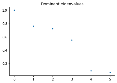
We expect four eigenvalues close to one. These dominant eigenvalues correspond to the slow dynamics. The eigenfunction of the Koopman operator associated with the eigenvalue $\lambda=1$ is the constant function, and the eigenfunction of the Perron-Frobenius operator associated with this eigenvalue is the invariant density.

d = np.real(kedmd_model.eigenvalues)
plt.plot(d, '.')
plt.title('Dominant eigenvalues');

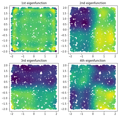
The eigenfunctions contain information about the metastable sets and slow transitions.

fig = plt.figure(figsize=(8, 8))
gs = fig.add_gridspec(ncols=2, nrows=2)

ax = fig.add_subplot(gs[0, 0])
ax.scatter(*X.T, c=phi[:, 0])
ax.set_title('1st eigenfunction')

ax = fig.add_subplot(gs[0, 1])
ax.scatter(*X.T, c=phi[:, 1])
ax.set_title('2nd eigenfunction')

ax = fig.add_subplot(gs[1, 0])
ax.scatter(*X.T, c=phi[:, 2])
ax.set_title('3rd eigenfunction')

ax = fig.add_subplot(gs[1, 1])
ax.scatter(*X.T, c=phi[:, 3])
ax.set_title('4th eigenfunction');

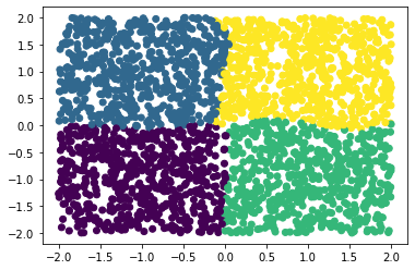
We can now apply clustering techniques to the dominant eigenfunctions to obtain metastable sets.

from deeptime.clustering import KMeans

kmeans = KMeans(n_clusters=4, n_jobs=4).fit(phi[:, :4]).fetch_model()
c = kmeans.transform(phi[:, :4])

plt.scatter(*X.T, c=c);

References

[1]

Matthew O Williams, Clarence W Rowley, and Ioannis G Kevrekidis. A kernel-based method for data-driven Koopman spectral analysis. Journal of Computational Dynamics, 2(2):247–265, 2015.

[2]

Stefan Klus, Ingmar Schuster, and Krikamol Muandet. Eigendecompositions of transfer operators in reproducing kernel Hilbert spaces. Journal of Nonlinear Science, 30:283–315, 2019. doi:10.1007/s00332-019-09574-z.

[3]

Stefan Klus, Andreas Bittracher, Ingmar Schuster, and Christof Schütte. A kernel-based approach to molecular conformation analysis. The Journal of Chemical Physics, 149(24):244109, 2018.