Kernel VAMP / kernel CCA

This notebook illustrates how to use kernel canonical correlation analysis (kernel CCA) [1] to compute coherent sets.

CCA [2] was originally developed to maximize the correlation between two multidimensional random variables \(X\) and \(Y\). Kernel CCA is a nonlinear variant of CCA, where the standard inner products are replaced by a kernel function \(k\) (using the well-known kernel trick). Popular kernel functions are the polynomial kernel \(k(x, x^\prime) = (c + x^\top x^\prime)^p\) and the Gaussian kernel \(k(x, x^\prime) = \exp(-\|x-x^\prime\|_2^2/2\sigma^2)\), see also deeptime.kernels. In our setting, \(Y\) is a time-lagged version of \(X\), i.e., we consider the process \(Y_t = X_{t + \tau}\). Here, \(\tau\) is a fixed lag time. The kernel CCA problem [1] can be written as an optimization problem of the form

\[\sup_{\substack{ f \in \mathbb{H}_X \\ g \in \mathbb{H}_Y }} \langle g, C_{YX} f \rangle_{\mathbb{H}_y} \quad \text{s.t.} \quad \begin{cases} \langle f, C_{XX} f\rangle_{\mathbb{H}_X} = 1, \\ \langle g, C_{YY} g\rangle_{\mathbb{H}_Y} = 1, \end{cases}\]

where \(C_{XX}\) and \(C_{YY}\) are covariance operators associated with \(X\) and \(Y\), respectively, and \(C_{YX}\) is the cross-covariance operator (these operators can be regarded as nonlinear versions of covariance and cross-covariance matrices). The solution of this optimization problem is given by the solution of a generalized eigenvalue problem, which can be simplified to

\[\big(C_{XX} + \varepsilon \mathcal{I}\big)^{-1} C_{XY} \big(C_{YY} + \varepsilon \mathcal{I}\big)^{-1} C_{YX} f = \rho^2 f.\]

Since the covariance operators are in general not invertible, we regularized the problem: \(\varepsilon\) is a regularization parameter and \(\mathcal{I}\) the identity operator. We estimate these operators using training data \(\{x_i\}_{i=1}^n\) and \(\{y_i\}_{i=1}^n\), where \(y_i\) is the time-lagged version of \(x_i\). Eigenfunctions of this operator eigenvalue problem can be found by solving an auxiliary matrix eigenvalue problem: Let \(G_{XX}\) and \(G_{YY}\) denote the Gram matrices with entries \([G_{XX}]_{ij} = k(x_i, x_j)\) and \([G_{YY}]_{ij} = k(y_i, y_j)\) and \(I\) the identity matrix. We solve

\[(G_{XX} + n \varepsilon I)^{-1} G_{XX} G_{YY} (G_{YY} + n \varepsilon I)^{-1} v = \rho^2 v\]

and obtain eigenfunctions \(f = \Phi v\), where \(\Phi = [k(x_1, \cdot), \dots, k(x_n, \cdot)]\) is the feature matrix associated with \(X\). There are many equivalent formulations, a detailed derivation can be found in [3].

Kernel CCA applied to Lagrangian data computes eigenfunctions of a dynamical operator associated with the forward-backward dynamics, which can be interpreted in terms of coherent sets as defined, e.g., in [4]. We will use the Bickley jet as a guiding example.

import numpy as np
import matplotlib.pyplot as plt

from IPython.display import HTML

First, we uniformly sample \(n\) data points in \(\mathbb{X} = [0, 20] \times [-3, 3]\). The domain is periodic in x-direction. The lag-time is defined to be \(\tau = 40\).

from deeptime.data import bickley_jet

n = 3000
bickley_data = bickley_jet(n_particles=n, n_jobs=8)
dataset = bickley_data.endpoints_dataset()

We choose the Gaussian kernel with bandwidth \(\sigma = 1\). Note that this kernel does not take the periodicity into account. However, the kernel could be easily adapted to be periodic in x-direction.

from deeptime.kernels import GaussianKernel

sigma = 1
kernel = GaussianKernel(sigma)

We then compute the first nine dominant eigenvalues and corresponding eigenvectors. The regularization parameter is set to \(\epsilon = 10^{-3}\).

from deeptime.decomposition import KernelCCA

kcca_estimator = KernelCCA(kernel, n_eigs=9, epsilon=1e-3)
kcca_model = kcca_estimator.fit((dataset.data, dataset.data_lagged)).fetch_model()
ev_real = np.real(kcca_model.eigenvectors)

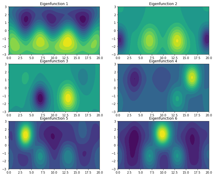
Let us visualize a few dominant eigenfunctions.

grid = np.meshgrid(np.linspace(0, 20, 150), np.linspace(-3, 3, 50))
xy = np.dstack(grid).reshape(-1, 2)
z = kcca_model.transform(xy).real

fig = plt.figure(figsize=(12, 10))
gs = fig.add_gridspec(ncols=2, nrows=3)

for row in range(3):
    for col in range(2):
        ix = col + 2*row
        ax = fig.add_subplot(gs[row, col])
        ax.contourf(grid[0], grid[1], z[:, ix].reshape(grid[0].shape), levels=15)
        ax.set_title(f"Eigenfunction {ix+1}")

The first eigenfunction distinguishes between the top and bottom half of the domain. The other eigenfunctions pick up combinations of the vortices.

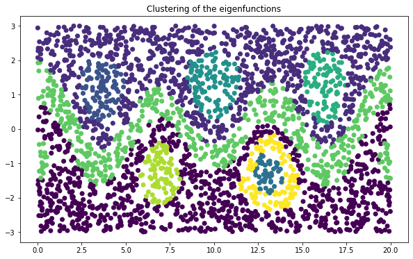
In order to find the corresponding coherent sets, we cluster the eigenvectors using \(k\)-means. Here, we compute 9 clusters.

from deeptime.clustering import KMeans

kmeans = KMeans(n_clusters=9, n_jobs=8).fit(ev_real).fetch_model()

Clustering of the dominant eigenfunctions results in the expected coherent sets.

plt.figure(figsize=(10, 6))
c = kmeans.transform(ev_real)
plt.scatter(*dataset.data.T, c=c)
plt.title('Clustering of the eigenfunctions')

Text(0.5, 1.0, 'Clustering of the eigenfunctions')

ani = bickley_data.make_animation(s=100, c=c/9, stride=2)
HTML(ani.to_html5_video())

It is also possible to optimize the kernel parameters for the VAMP-2 score using standard optimization tools. To this end, we define an objective function:

from deeptime.decomposition import vamp_score_data

# we only use the first 500 datapoints for the sake of runtime
opt_data = dataset.data[:500]
opt_data_lagged = dataset.data_lagged[:500]

def objective(params):
    bandwidth, epsilon = params
    kernel = GaussianKernel(bandwidth)
    kcca = KernelCCA(kernel, n_eigs=9, epsilon=epsilon).fit((opt_data, opt_data_lagged))
    kcca_model = kcca.fetch_model()
    # we only use the real part
    transform = lambda x: kcca_model.transform(x).real
    return -vamp_score_data(dataset.data, dataset.data_lagged, transform, r=2)

The objective function takes bandwidth and regularization and estimates a kCCA model based on that, subsequently computing a VAMP-2 score on kCCA-transformed data.

Now, we can use SciPy to optimize bandwidth and epsilon.

from scipy.optimize import minimize, Bounds

# bandwidth no smaller than 1e-3, epsilon no smaller than 1e-3
bounds = Bounds([1e-1, 1e-3], [np.inf, np.inf])
result = minimize(objective, x0=[1.0, 1e-2], bounds=bounds, method='SLSQP')

bw_opt, eps_opt = result.x
print(f"Optimization successful={result.success} with "
      f"bandwidth={bw_opt.round(2)} and epsilon={eps_opt.round(2)}")
print(f"Optimized score {-objective((bw_opt, eps_opt)).round(2)} vs. "
      f"guessed score {-objective((kcca_estimator.kernel.sigma, kcca_estimator.epsilon)).round(2)}")

/home/mho/miniconda3/envs/deeptime/lib/python3.9/site-packages/scipy/optimize/optimize.py:282: RuntimeWarning: Values in x were outside bounds during a minimize step, clipping to bounds
  warnings.warn("Values in x were outside bounds during a "

Optimization successful=True with bandwidth=0.62 and epsilon=0.0
Optimized score 5.26 vs. guessed score 4.68

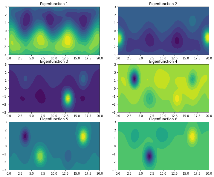
With optimized bandwidth and epsilon, we can again evaluate, e.g., the first eigenfunctions.

kcca_opt = KernelCCA(GaussianKernel(bw_opt), n_eigs=9, epsilon=eps_opt) \
    .fit((dataset.data, dataset.data_lagged)).fetch_model()

grid = np.meshgrid(np.linspace(0, 20, 150), np.linspace(-3, 3, 50))
xy = np.dstack(grid).reshape(-1, 2)
z = kcca_opt.transform(xy).real

fig = plt.figure(figsize=(12, 10))
gs = fig.add_gridspec(ncols=2, nrows=3)

for row in range(3):
    for col in range(2):
        ix = col + 2*row
        ax = fig.add_subplot(gs[row, col])
        ax.contourf(grid[0], grid[1], z[:, ix].reshape(grid[0].shape), levels=15)
        ax.set_title(f"Eigenfunction {ix+1}")

References

[1] (1,2)

Francis R Bach and Michael I Jordan. Kernel independent component analysis. Journal of machine learning research, 3(Jul):1–48, 2002.

[2]

Harold Hotelling. Relations between two sets of variates. In Breakthroughs in statistics, pages 162–190. Springer, 1992.

[3]

Stefan Klus, Brooke E Husic, Mattes Mollenhauer, and Frank Noé. Kernel methods for detecting coherent structures in dynamical data. Chaos, 2019. doi:10.1063/1.5100267.

[4]

Gary Froyland, Naratip Santitissadeekorn, and Adam Monahan. Transport in time-dependent dynamical systems: finite-time coherent sets. Chaos: An Interdisciplinary Journal of Nonlinear Science, 20(4):043116, 2010. doi:10.1063/1.3502450.