function swissroll_model

deeptime.data.swissroll_model(n_samples, seed=None)

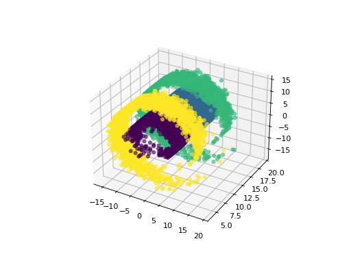
Sample a hidden state and an swissroll-transformed emission trajectory, so that the states are not linearly separable.

(Source code, png, hires.png, pdf)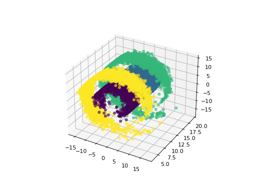

Parameters:

• n_samples (int) – Number of samples to produce.

• seed (int, optional, default=None) – Random seed to use. Defaults to None, which means that the random device will be default-initialized.

Returns:

• sequence ((n_samples, ) ndarray) – The discrete states.

• trajectory ((n_samples, ) ndarray) – The observable.

Notes

First, the hidden discrete-state trajectory is simulated. Its transition matrix is given by

$$P = \begin{pmatrix}0.95 & 0.05 & & \\ 0.05 & 0.90 & 0.05 & \\ & 0.05 & 0.90 & 0.05 \\ & & 0.05 & 0.95 \end{pmatrix}.$$

The observations are generated via the means are $\mu_0 = (7.5, 7.5)^\top$, $\mu_1= (7.5, 15)^\top$, $\mu_2 = (15, 15)^\top$, and $\mu_3 = (15, 7.5)^\top$, respectively, as well as the covariance matrix

$$C = \begin{pmatrix} 1 & 0 \\ 0 & 1 \end{pmatrix}.$$

Afterwards, the trajectory is transformed via

$$(x, y) \mapsto (x \cos (x), y, x \sin (x))^\top.$$