function abc_flow¶

deeptime.data.abc_flow(h=0.001, n_steps=10000)¶

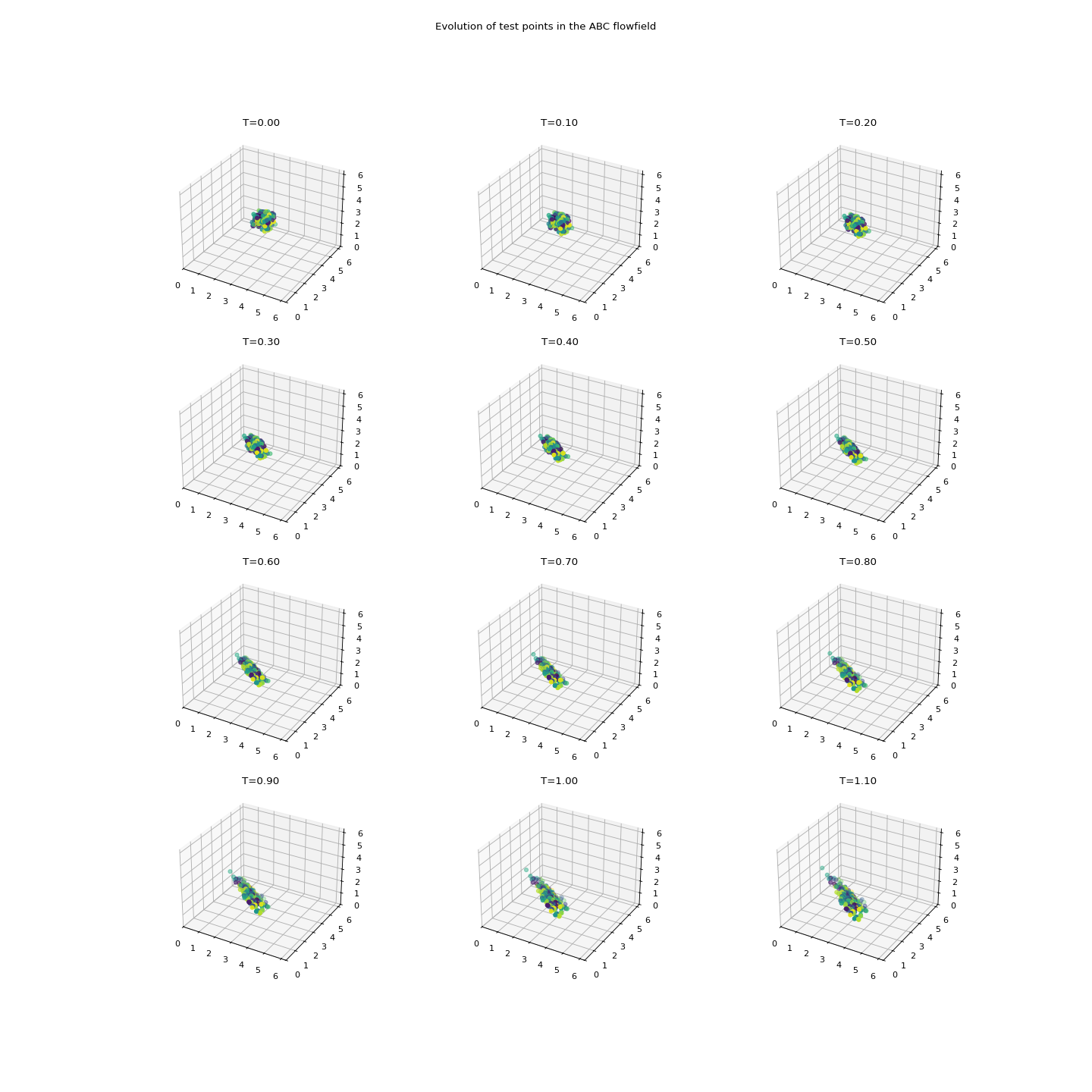
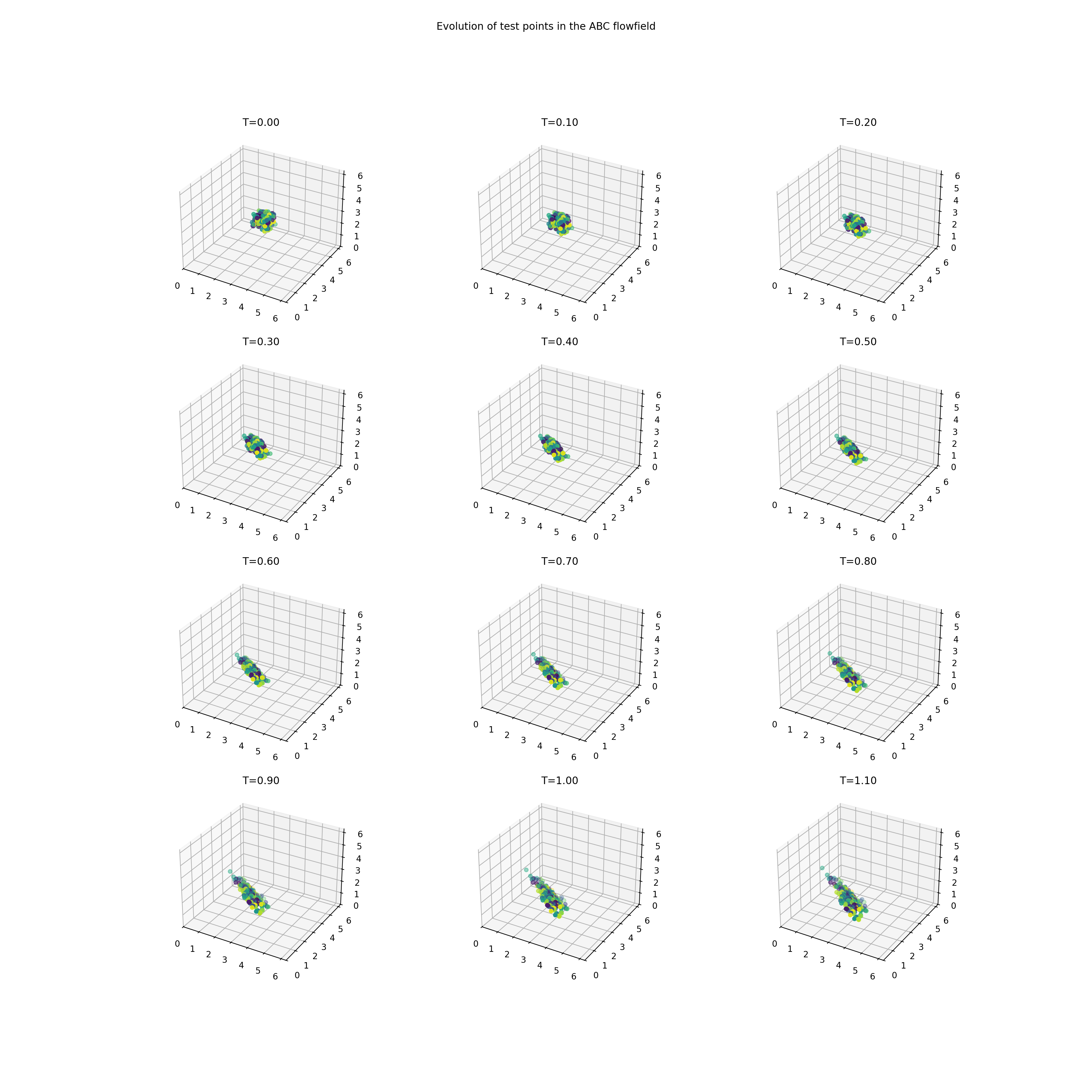
The Arnold-Beltrami-Childress flow. [1] It is generated by the ODE

\begin{aligned} \dot{x} &= A\sin(z) + C\cos(y)\\ \dot{y} &= B\sin(x) + A\cos(z)\\ \dot{z} &= C\sin(y) + B\cos(x) \end{aligned}

on the domain $\Omega=[0, 2\pi]^3$ with the parameters $A=\sqrt{3}$ , $B=\sqrt{2}$ , and $C=1$ .

(Source code, png, hires.png, pdf)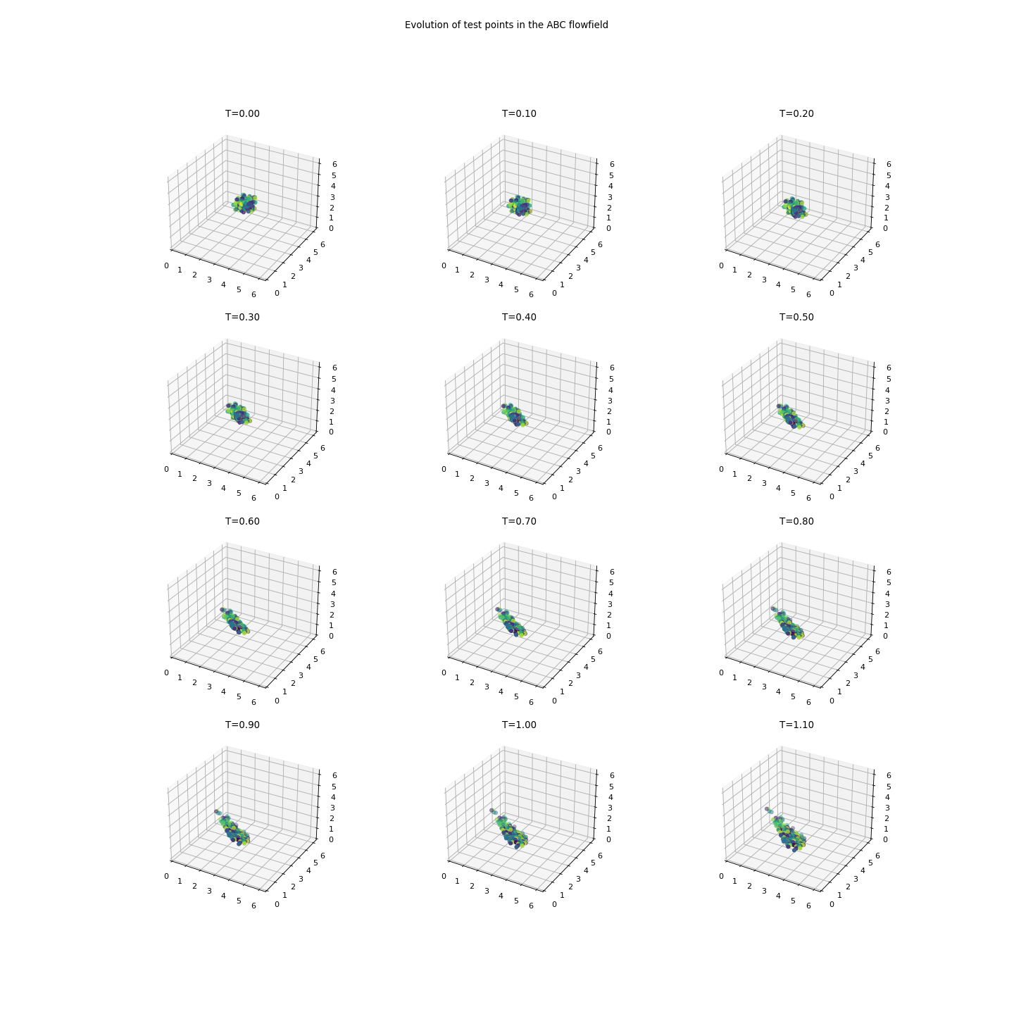

../../_images/deeptime-data-abc_flow-1.png

Parameters:

h (float, default = 1e-3) – Integration step size. The implementation uses an Runge-Kutta integrator.
n_steps (int, default = 10000) – Number of integration steps between each evaluation. That means the default lag time is h*n_steps=10.

Returns:

system – The system.

Return type:

TimeIndependentSystem

Examples

The model possesses the capability to simulate trajectories as well as be evaluated at test points:

>>> import numpy as np
>>> import deeptime as dt

First, set up the model (which internally already creates the integrator).

>>> model = dt.data.abc_flow(h=1e-3, n_steps=100)  # create model instance

Now, a trajectory can be generated:

>>> traj = model.trajectory(np.array([[-1., 0., 0.]]), 1000, seed=42, n_jobs=1)  # simulate trajectory
>>> assert traj.shape == (1000, 3)  # 1000 evaluations from initial condition [0, 0]

Or, alternatively the model can be evaluated at test points (mapping forward using the dynamical system):

>>> test_points = np.random.uniform(.5, 1.5, (100, 3))  # 100 test points
>>> evaluations = model(test_points, seed=53, n_jobs=1)
>>> assert evaluations.shape == (100, 3)

References